Thermal Management of a Graphics Processing Unit (GPU)
A study on forced convection and conjugate heat transfer in PCB assemblies, covering the Navier-Stokes equations, energy conservation, and numerical modeling in Ansys Icepak.
Conjugate Heat Transfer in Electronics
Electronics cooling is a classic Conjugate Heat Transfer (CHT) problem, where heat is transferred via conduction through solid components (silicon chips, FR4 PCB) and subsequently removed by a moving fluid (air) through convection.
In this project, a high-power AGP chip was modeled with an aluminum-extruded heatsink and a forced-air fan system to solve the coupled behavior of fluid flow and solid temperature distribution.
The simulation model represents a high-performance PCB assembly designed in Fusion 360 and analyzed in Ansys Icepak. The system consists of several critical heat-generating modules, each serving a distinct functional role:
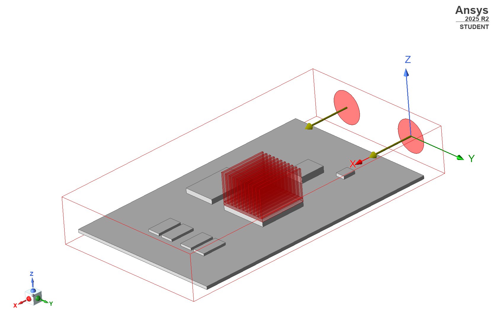
(a) Electonics GPU Model
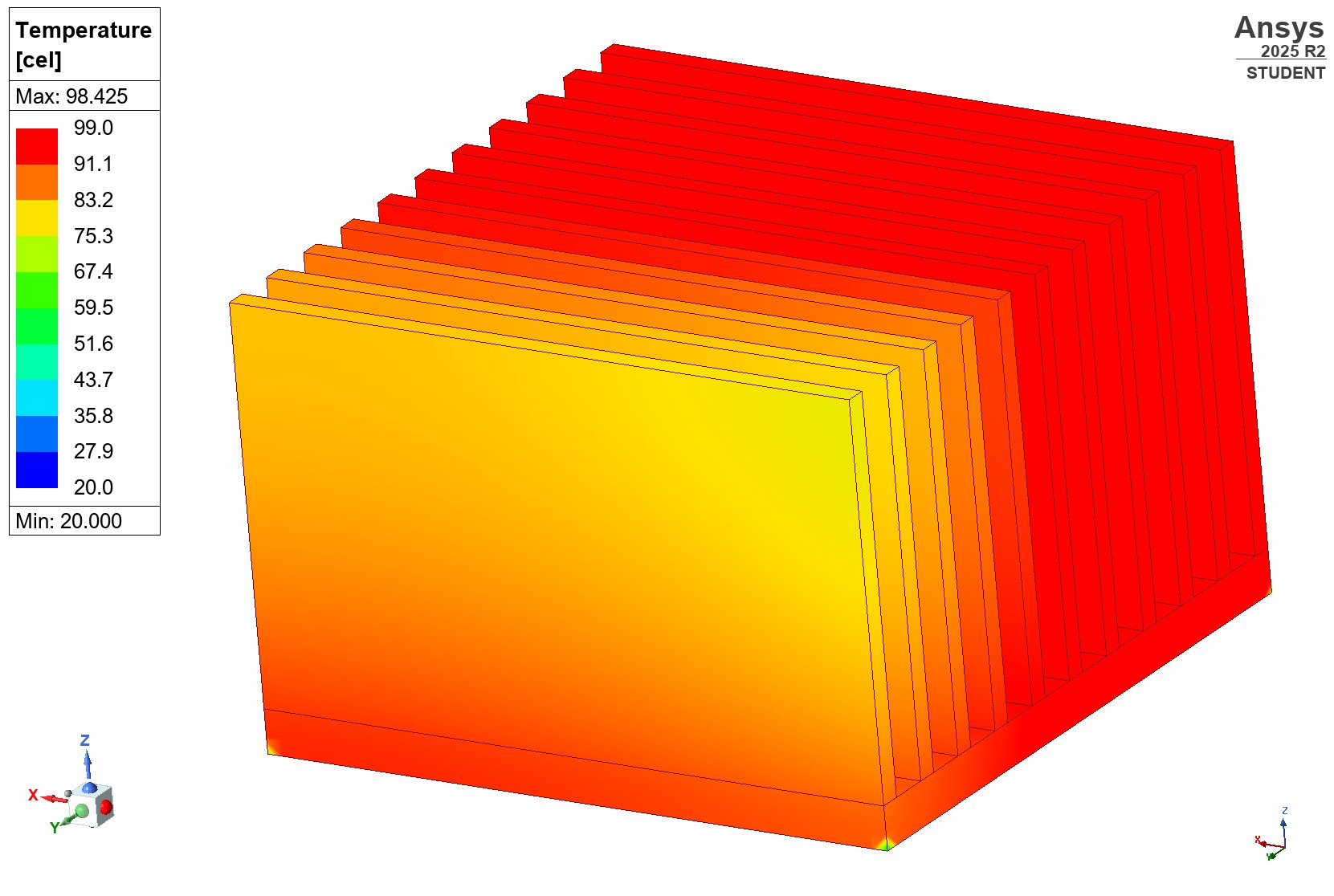
(b) Heatsink Temperature Map
- AGP (Accelerated Graphics Port) Chip: The primary processing unit and main heat source, generating a significant thermal load of 54W.
- DDR (Double Data Rate) Modules: Four separate memory bodies responsible for high-speed data buffering, each contributing a localized heat flux of 4.5W.
- Bridge and Flash Chips: Secondary logic components that manage data flow and storage, requiring thermal monitoring to prevent localized hot spots.
- Aluminum Heatsink: An extruded fin-base structure designed to maximize the surface area for convective heat transfer.
- Forced-Air Fans: Two axial fans that drive airflow across the components to break down the thermal boundary layer.
Governing Equations
To simulate the airflow, Icepak solves the Navier-Stokes equations, which describe the conservation of mass and momentum for a Newtonian fluid:
Continuity Equation (Mass Conservation)
\[\nabla \cdot \mathbf{u} = 0\]Momentum Equation (Newton’s Second Law for Fluids)
\[\rho \left( \frac{\partial \mathbf{u}}{\partial t} + \mathbf{u} \cdot \nabla \mathbf{u} \right) = -\nabla p + \mu \nabla^2 \mathbf{u} + \mathbf{f}\]Where $\mathbf{u}$ is the velocity vector, $\rho$ is the density of air, $p$ is the pressure, and $\mu$ is the dynamic viscosity.
The Energy Equation
The temperature distribution across the PCB and through the cooling fins is governed by the energy equation:
\[\rho C_p \left( \frac{\partial T}{\partial t} + \mathbf{u} \cdot \nabla T \right) = \nabla \cdot (k \nabla T) + \dot{q}\]where:
- $k$ is the thermal conductivity (e.g., $k \approx 200 \text{ W/m}\cdot\text{K}$ for Aluminum).
- $\dot{q}$ is the volumetric heat source (e.g., the 54W load on the AGP chip).
Modeling Forced Convection
To achieve high accuracy, the simulation utilizes several specialized modeling techniques within the Ansys Icepak environment.
Optimized Mesh and Elements
The model utilizes a fine meshing strategy with a total count of approximately 500,000 elements. Icepak-optimized objects are employed to handle complex geometries efficiently:
- Heatsink Elements: The mesh is locally refined between the fins to capture the high-velocity gradients and wake effects.
- Fan Objects: Specialized Icepak fan objects are used to accurately model the swirl and pressure-jump characteristics of air entering the system.
- Non-Conformal Meshing: This allows for a dense mesh around critical components like the AGP chip while maintaining a coarser, computationally efficient mesh in the ambient air region.
Thermal Network Definitions
For the AGP and Bridge components, we move beyond simple solid blocks to a Circuit Model (Two-Resistor Model) approach. This defines the thermal path using:
- Junction-to-Case ($R_{jc}$) resistance.
- Junction-to-Board ($R_{jb}$) resistance.
- Thermal Interface Materials (TIM): Two distinct thermal interfacial resistances are applied to model the contact between the chip surface and the heatsink, ensuring realistic heat conduction paths that account for microscopic air gaps and material imperfections.
Turbulence Modeling
The fluid dynamics are solved using a two-equation turbulence model (such as $k-\epsilon$ or $k-\omega$). This approach provides the necessary fidelity to resolve the turbulent kinetic energy and dissipation rates as air moves through the restricted channels of the heatsink fins.
Transient Thermal Analysis
The following results visualize the final thermal state and the transient journey of the GPU assembly under a 350-second operational load.
1. Steady-State Temperature Distribution
The final temperature contour reveals a maximum temperature of 123.48°C, localized at the AGP junction. A closer inspection of the heatsink shows a peak temperature of 98.43°C at its base. The speed contour illustrates the effectiveness of the dual-fan setup. Air reaches a maximum velocity of 15.65 m/s at the fan exhaust.
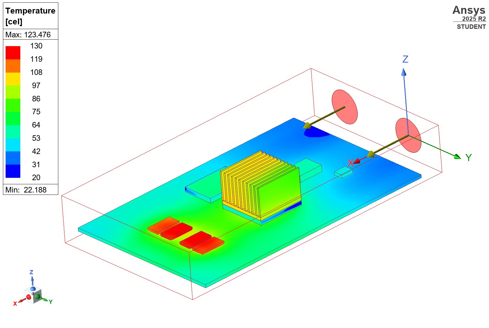
(a) Full PCB Surface Temperature
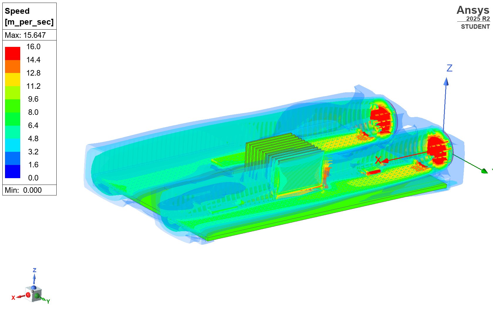
(b) Velocity Fields
The heatsink effectively pulls heat away from the AGP, as evidenced by the temperature gradient across the fins (ranging from ~98°C at the base to lower temperatures at the tips). The surrounding DDR modules also show significant thermal elevation, necessitating their inclusion in the forced-convection path.
2. Convergence and Residuals
The “Monitor Temperature” plot tracks the real-time heating of individual components. The numerical health of the simulation is confirmed by the Residual Plot.
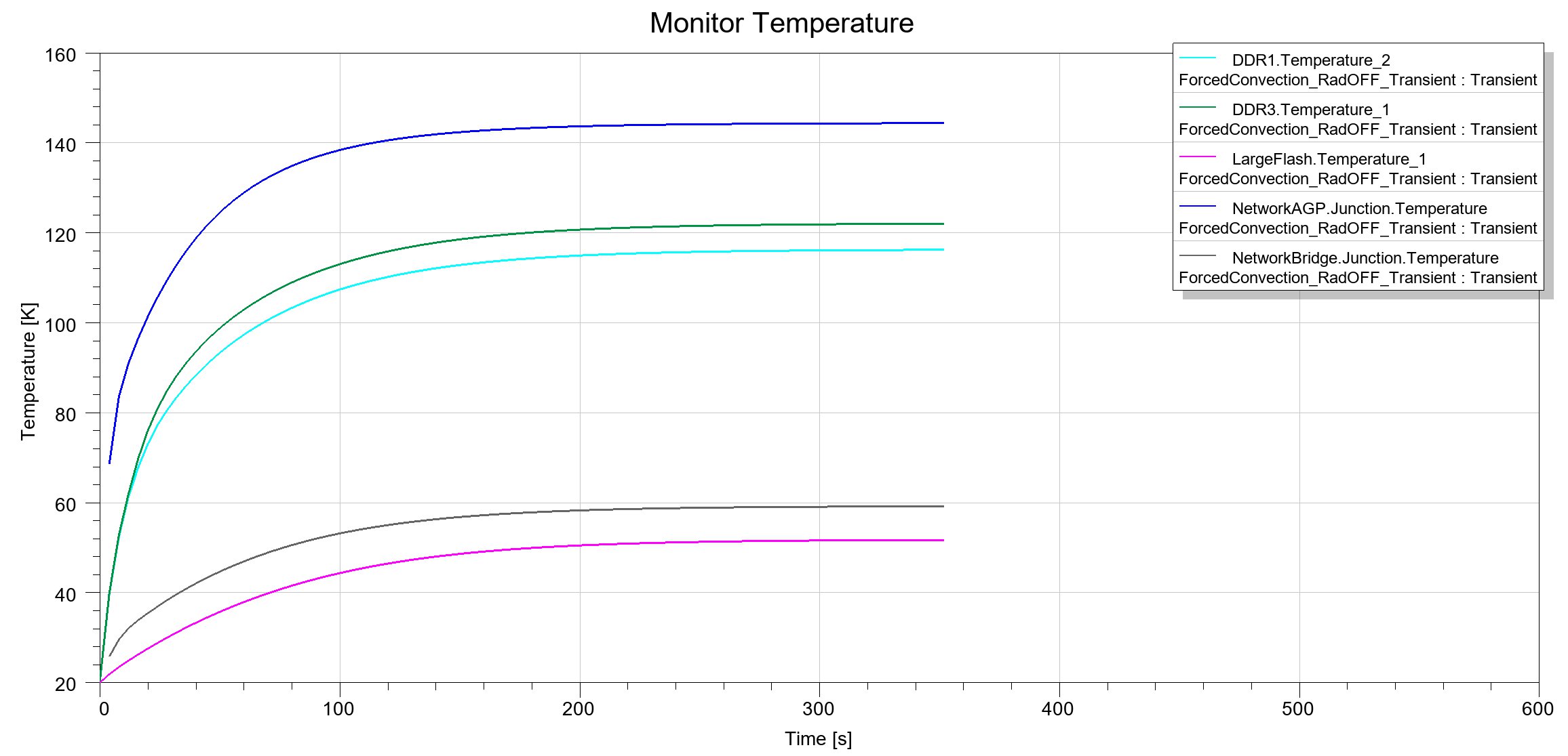
(a) Temperature Monitor
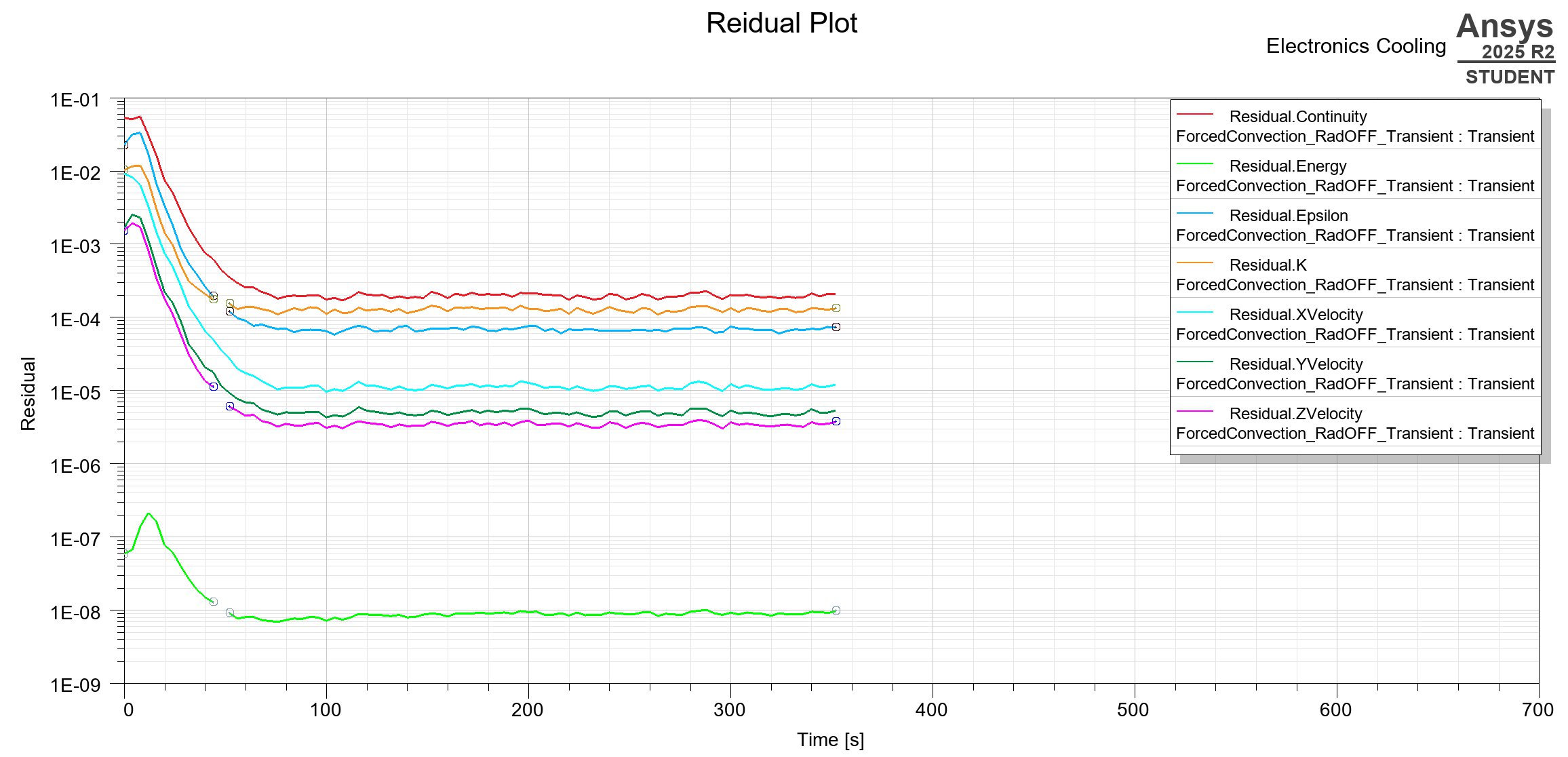
(b) Velocity Fields
- AGP Junction: Exhibits the steepest rise, stabilizing near 145 K above ambient.
- DDR Modules: Follow a similar curve but plateau lower, reflecting their lower power density.
- Bridge/Flash: Maintain significantly lower temperatures, indicating that the cooling solution is more than adequate for these secondary components.
Specifically, the Energy residual (green line) dropped to the 1E-08 range, which is well below the standard 1E-07 requirement for electronics cooling. The stability of the velocity residuals ($X, Y, Z$) confirms that the two-equation turbulence model successfully resolved the complex flow through the heatsink fins without oscillating or diverging.