PINNs

Leveraging Physics-Informed Neural Networks (PINNs) for solving scientific PDEs

2D Heat Equation

In the case of the 2D heat equation, which describes how heat diffuses through a two-dimensional surface over time, a PINN can learn the temperature distribution across space and time by minimizing the residual of the heat equation at sampled points in the domain.

\[\frac{\partial u}{\partial t} = \alpha \left( \frac{\partial^2 u}{\partial x^2} + \frac{\partial^2 u}{\partial y^2} \right), \quad (x, y) \in \Omega, \ t > 0\]

Futhermore, we consider the following initial condision and boundary conditions for the system,

\[u(x, y, 0) = sin(\pi x) sin(\pi y), \quad (x, y) \in \Omega \\ \\\] \[u(x, 1, t) = 1, \quad u(x, y, t) = 0, \quad (x, y) \in \partial \Omega, \ t > 0\]

What is Physics-Informed Neural Network (PINN)?

In simple terms, machine learning for science equations(but not limited to it). A Physics-Informed Neural Network (PINN) is a type of deep learning model that incorporates physical laws—typically expressed as partial differential equations (PDEs)—directly into the training process of the neural network. Unlike traditional neural networks that rely solely on labeled data, PINNs are trained using both data (if available) and the governing physical equations, enabling them to learn accurate solutions even with limited or no data.

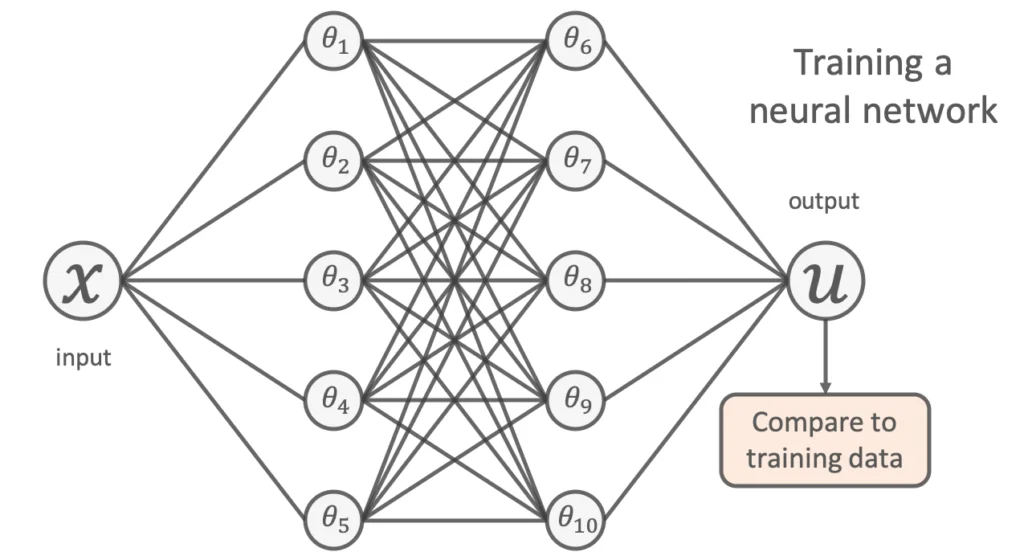
To learn a model, we try to tune the network’s free parameters (denoted by the \thetas in the figure above) so that the network’s predictions closely match the available experimental data. This is usually done by minimising the mean-squared-error between its predictions and the training points;

\[\begin{align} \min \frac{1}{N} \sum_{i=1}^{N} \left( u_{\text{NN}}(x_i; \theta) - u_{\text{true}}(x_i) \right)^2 \end{align}\]

Julia Implementation and Code Walkthrough

We use NeuralPDE.jl for defining and solving PDEs, Lux.jl for neural networks, and ModelingToolkit.jl for symbolic definitions. We symbolically define the time and space variables along with their partial derivatives.

using NeuralPDE, Lux, Optimization, OptimizationOptimJL
using ModelingToolkit: Interval

@parameters t, x, y
@variables u(..)
Dx = Differential(x); Dy = Differential(y); Dt = Differential(t)
Dxx = Dx^2; Dyy = Dy^2

Next, define the complete PDE system including equations and constraints.

α = 1.0
eq = Dt(u(t, x, y)) ~ α * (Dxx(u(t, x, y)) + Dyy(u(t, x, y)))
domains = [
    t ∈ Interval(0.0, 1.0),
    x ∈ Interval(0.0, 1.0),
    y ∈ Interval(0.0, 1.0)
]
ic = u(0, x, y) ~ 0
bcs = [
    u(t, 0, y) ~ 0.0,
    u(t, 1, y) ~ 0.0,
    u(t, x, 0) ~ 0.0,
    u(t, x, 1) ~ 1.0
]
@named pde_system = PDESystem(eq, [ic; bcs], domains, [t, x, y], [u(t, x, y)])

Finally, set up and trains the Physics-Informed Neural Network (PINN) to solve the 2D heat equation. It defines the neural network architecture, discretizes the PDE using grid-based training, and initializes the optimization problem. Training is performed using the ADAM optimizer with a callback to monitor loss, and the final trained model can be used to predict the solution over the domain.

dx = 0.05
chain = Chain(Dense(3, 32, tanh), Dense(32, 32, tanh), Dense(32, 1))
discretization = PhysicsInformedNN(chain, GridTraining(dx))
prob = discretize(pde_system, discretization)
losses = []

callback = function (p, l)
    println("Current loss is: $l")
    push!(losses, l)
    return false
end
using OptimizationOptimisers
opt1 = OptimizationOptimisers.Adam(0.01)
res1 = Optimization.solve(prob, opt1; callback=callback, maxiters=1000)
phi = discretization.phi

xs = ys = range(0, 1, length=50)
t_plot = 0.0  # Fixed time
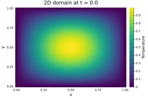
u_predict = [sin(pi*x)*sin(pi*y) for x in xs, y in ys]
heatmap(xs, ys, u_predict', xlabel="x", ylabel="y", title="2D domain at t = $t_plot", 
        color=:viridis, colorbar=true, colorbar_title="Temperature")
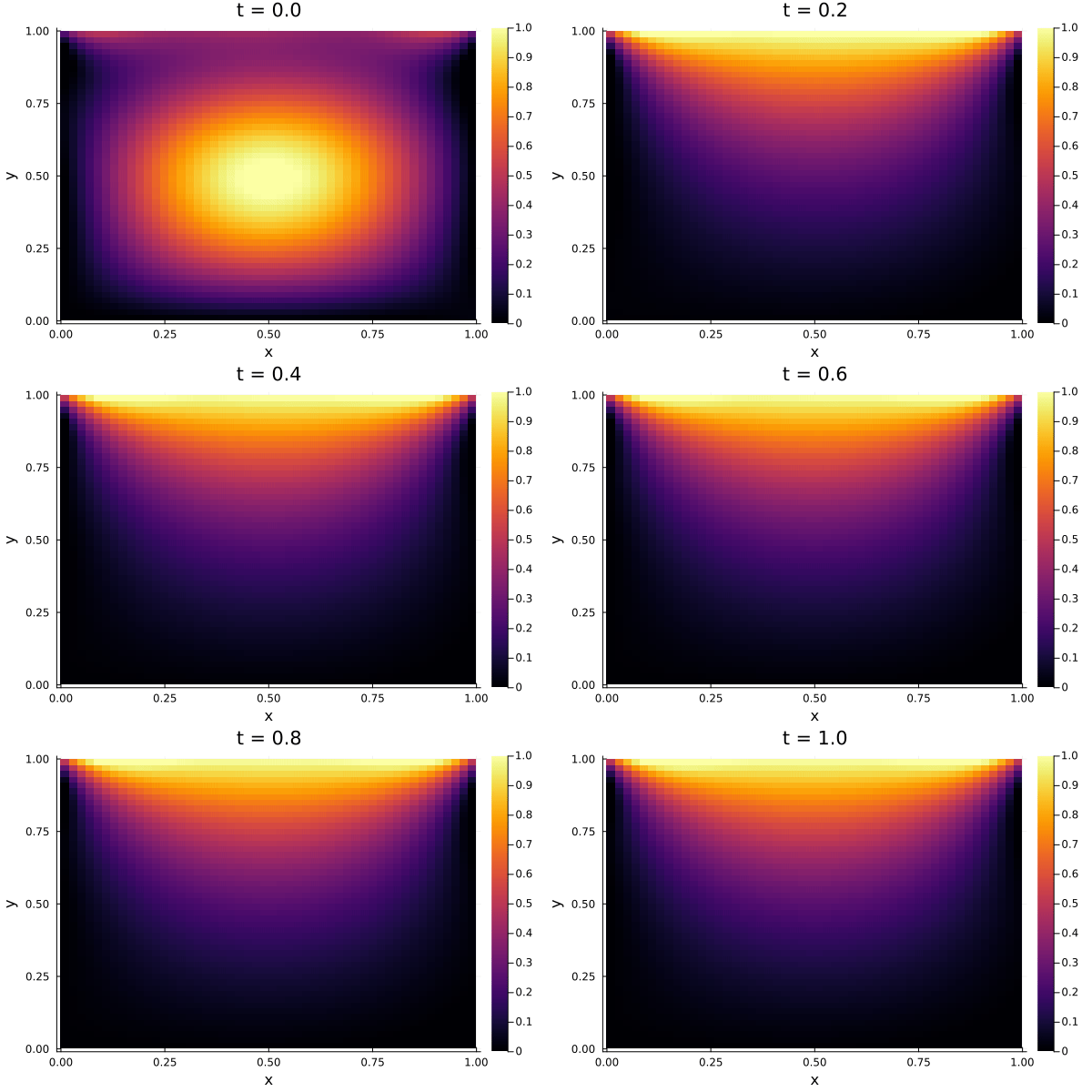
anim = @animate for t_plot in 0:0.005:1.0
    u = [phi([t_plot, x, y], res.u)[1] for x in xs, y in ys]
    heatmap(0:0.02:1, 0:0.02:1, u', title="t = $t_plot", xlabel="x", ylabel="y", clims=(0,1))
end
gif(anim, "newheat2d.gif", fps=10)
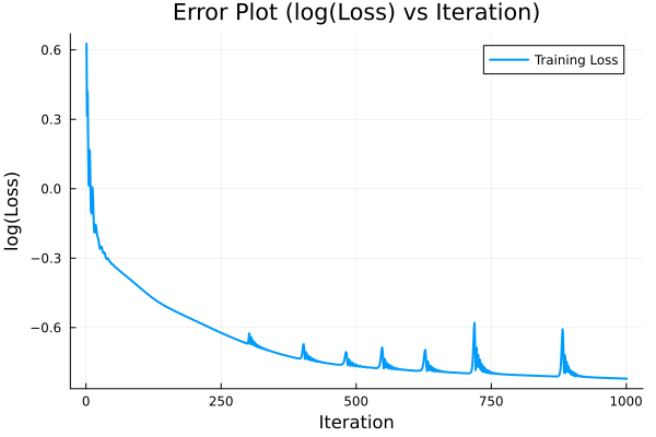
plot(1:length(losses), log10.(losses),
    xlabel="Iteration", ylabel="log(Loss)",
    title="Error Plot (log(Loss) vs Iteration)",
    label="Training Loss", linewidth=2)

After training the PINN model, we can visualize its predictions over time and space. The following Julia code uses the Plots.jl library to create both static heatmaps and animated GIFs showing the temperature evolution in the 2D domain.

---

Initial temperature distribution heat map we start with:

Temperature field from our PINN network develops as follows:

Error plot over time:

—